Counting orbit points under group actions - Part 1

After 10 months of being unable to come up with anything interesting to post on the blog, I realized it might be a good idea use this blog to keep track of the math I've been working on. That way my blog can act as a public version of my research notebook, and be a good place to relearn this material if I happen to forget the details in the future.

I have been learning some Patterson-Sullivan theory for the past few weeks with the goal of using the theory to solve some counting problems. To be more precise, I'm working with the following setup.

• \(X\) is an unbounded metric space (in practice, \(X\) is usually \(\mathbb{R}^n\), \(\mathbb{H}^n\), or \(\mathcal{T}_{g}\) (the Teichmüller space of genus \(g\) surfaces)).
• \(\Gamma\) is a discrete group acting on \(X\) via isometries.

Given a point \(x \in X\), and a radius \(r\), I'm interested in knowing how many points of the orbit of \(x\) under \(\Gamma\), which we'll denote \(\Gamma x\), lie in a ball of radius \(r\) about \(x\) (which we'll denote by \(B(x, r)\)). Since we're dealing with a discrete group, the number of orbit points clearly won't be a continuous function of \(r\), which means we can't expect a nice exact answer, but we can ask questions about the asymptotics of the orbit counting function.

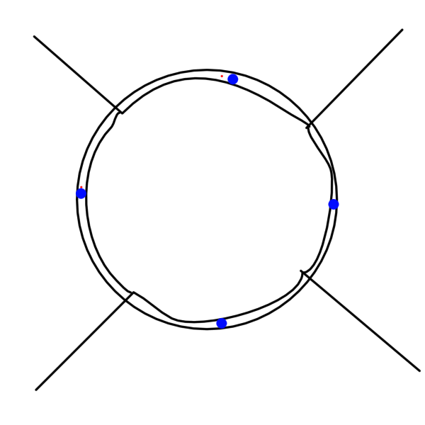
It's instructive to start off with the simplest example: our metric space is \(\mathbb{R}^2\), and our discrete group \(\Gamma\) is just the group generated by translations by \((0,1)\) and \((1,0)\). If we pick \(x\) to be the point \((0.5,0.5)\) (we're picking this point so our pictures look nicer), our orbit counting question translates to the following question: How many half-integer points does a ball of radius \(r\) contain? A way to answer this question is to think of the fundamental domain of the group \(\Gamma\). If the ball contains \(n\) points, we might expect it to contain \(n\) copies of the fundamental domain, which means we'd expect it have \(n\) times the area of a fundamental domain. That's not quite correct, as the following picture demonstrates.

Figure 1: The black orbit points have their fundamental domains completely in the ball, whereas the red ones don't. The ball also has parts of fundamental domains for which it doesn't contain the corresponding orbit point.

However, since the fundamental domain has diameter bounded by \(1\), we can expand and contract our ball slightly to get upper and lower bounds in terms of area. If we denote the number of orbit points in a ball of radius \(r\) as \(C(r)\), we get the following inequality for \(C(r)\).

Note now for large values of \(r\), \(\text{Area}(x, r-1)\) is approximately equal to \(\text{Area}(x, r+1)\), i.e. their ratio approaches \(0\). That means for large values of \(r\), \(C(r)\) behaves like \(\frac{\text{Area}(B(x, r+1))}{\text{Area}(\text{Fundamental domain})}\). This only works out because \(\frac{(r+1)^2}{(r-1)^2}\) approaches \(1\) as \(r\) gets larger.

The result in the case of \(\mathbb{R}^n\) suggests what the answer should be even in the more general cases, at least when the discrete group \(\Gamma\) has a fundamental domain with finite volume, i.e. when \(\Gamma\) is a lattice. In the case when one is working in \(\mathbb{H}^n\), the asymptotics are the same.

One might try the same proof as before, and it almost works except that it fails at a rather critical step. Recall that the volume of a ball of radius \(r\) in \(\mathbb{H}^n\) is not polynomial in \(r\), but rather exponential. To be more specific, the volume is proportional to \(e^r\), which means the following ratio does not converge to \(1\).

To be more precise, the thing that can go wrong is the following: by estimating the number of lattice points as \(c \cdot \text{Area}(B(x,r))\) (where \(c = \frac{1}{\text{Area}(\text{Fundamental domain})}\)), we may drastically over count or under count, as the following pictures illustrate.

Figure 2: This is an underestimate because even though the blue orbit points are in the ball, most of their fundamental domains aren't, which leads to an underestimate by the area calculation/

Figure 3: This is an overestimate because even though the blue orbit points are outside the ball, most of their fundamental domains are in the ball, which leads to an overestimate by the area calculation/

However, these are the worst case scenarios. In a more realistic scenario, one might expect the overestimates and underestimates to cancel out as the ball gets larger and larger. One might expect that to happen if the direction at which the boundary of the ball approaches translates of the fundamental domain is approximately random, and independent of the directions it approaches other translates by. That turns out to be true, and is a consequence of the fact that the geodesic flow on hyperbolic surfaces of finite volume is mixing. This intuition is formalized in the following lemma from a paper by Eskin and McMullen¹.

Lemma: Let \(X = \Gamma/\mathbb{H}^2\) be a finite volume hyperbolic surface, and \(S(p, r)\) be the image of a sphere of radius \(r\) on \(\mathbb{H}^2\) with centre a lift of a point \(p\) in \(\Gamma/\mathbb{H}^2\). Then for any compactly supported continuous function \(\alpha\), the average of \(\alpha\) over \(S(p, r)\) (with respect to the Lebesgue measure on \(S^1\)) approaches the average of \(\alpha\) over \(X\) as \(r\) approaches \(\infty\).

Proof: To prove this result, we need to lift the function \(\alpha\) to the unit tangent bundle \(T^1X\), and we do that in the obvious way, i.e. \({\alpha}(x, v) = \alpha(x)\), for any unit tangent vector \(v\) over \(x\). Also, let \(K\) be the set of all vectors over \(p\). Then the image of \(K\) under the geodesic flow \(g_t\) is the collection of vectors over \(S(p, t)\) pointing normally outwards. In particular, the average of \(\alpha\) over \(S(p, t)\) is the same as the average of \(\alpha\) over \(g_t(K)\)². Furthermore, \(g_t(K)\) can be approximated arbitrarily well by \(g_t(U)\) where \(U\) is the collection of vectors over a small neighbourhood of \(p\). Because the geodesic flow is mixing, the average of \(\alpha\) over \(g_t(U)\) approaches the average of \(\alpha\) over \(S^1X\) (and equivalently, \(X\)), as \(t\) approaches \(\infty\). This proves the result. \(\square\)

Once we have the lemma, the rest is smooth sailing. We let \(\alpha\) be a bump function supported in a small neighbourhood of \(p\), and lift \(\alpha\) to a function \(\widetilde{\alpha}\) on the universal cover. To count the number of orbit points in a ball of radius \(r\), we just integrate \(\widetilde{\alpha}\) on that ball. We can approximate this integral for large \(r\) using the lemma we just proved, and that gives us the estimate we want, namely that the number of orbit points in a ball of radius \(r\) is asymptotically \(\frac{\text{Area}(B(p, r))}{\text{Area}(\text{Fundamental Domain})}\).

One of the key elements of this proof was the fact that the geodesic flow is mixing with respect to a suitable measure. That suggests how one might extend this idea to other contexts. One important generalization of cocompact lattices are convex cocompact groups³. And for these groups, the estimates we have here don't work verbatim because the fundamental domain for a convex cocompact group may not have finite area. Secondly, the lemma as stated won't work either because the Liouville measure is not the "correct" measure on the unit tangent bundle. Not only is it not mixing, it's not even preserved by geodesic flow. In fact, the geodesic flow makes all the mass of Liouville measure escape the convex core, which means that one cannot do dynamics on a convex cocompact group using the Liouville measure. The right measure for this context turns out to be the Bowen-Margulis measure, which is constructed using the Patterson-Sullivan measure on the boundary, and that is what I will write about in my next blog post.

UPDATE: Part 2 of this series is up.