Counting orbit points (part 2): Patterson-Sullivan theory
Posted: Sun 05 January 2020Filed under mathematics
Tags: geometry dynamics topology
In the previous post, we saw how to get an asymptotic count of orbit points under a lattice action, i.e. a finite covolume Fuchsian group. To do so, we needed the fact that the geodesic flow on the associated quotient was mixing with respect to the Liouville measure. That suggests that if we want to get asymptotic counting for the orbit of an infinite covolume Fuchsian group, we might want to show mixing of the geodesic flow for the associated quotient space. However, proving mixing with respect to the Liouville measure is pointless, since the Liouville measure is infinite. What we need therefore, is a some other measure on the unit tangent bundle that is invariant under and mixing with respect to the geodesic flow.
For a class of Fuchsian groups known as geometrically finite groups, such a measure does exist: it's called the Bowen-Margulis measure. The construction of this measure is fairly involved, and will take up several blog posts, but the intermediate constructions are interesting in their own right. We will start off by looking at a family of measures associated to a geometrically finite group \(\Gamma\) on the limit set \(\Lambda(\Gamma)\), which is a subset of the boundary \(\partial \mathbb{H}^2\). These measures are called the Patterson-Sullivan measures.
Before we describe how the Patterson-Sullivan measures on the boundary are constructed, it will be useful to make explicit what properties we would like for them to have. We want this measure to respect the dimension of the limit set, at least infinitesimally. What that means is that if there's set of radius \(r\) which has measure \(\mu\), and if it's size is doubled to \(2r\), then it's measure should becomes \(2^\delta\) times the original measure, where \(\delta\) in some sense is the dimension of the limit set. In other words, whatever measure we construct on the limit set has to be compatible with the metric on the limit set.
Note however that the boundary \(\partial \mathbb{H}^2\) (and the limit set \(\Lambda(\Gamma)\) by extension), doesn't have a canonical metric. Instead, it has a family of metrics, all conformal to each other, and every one of those metrics come from a point \(x \in \mathbb{H}^2\). The metric associated to each point \(x\) comes from the identification of the unit tangent sphere at that point to the boundary. Suppose we did have a family of measures \(\mu_x\) one for each point, that satisfied the scaling property. That would then mean that for any two points \(x\) and \(y\), \(\mu_x\) was absolutely continuous with respect to \(\mu_y\) (and the other way round), and the Radon-Nikodym derivative \(\frac{d\mu_y}{d\mu_x}\) would be \(\left( \frac{g_y}{g_x} \right)^{\delta}\), where \(g_y\) and \(g_x\) are the associated metrics. For negatively curved spaces, the ratio \(\left( \frac{g_y}{g_x} \right)\) at a point \(\xi\) in the boundary is actually the Busemann function \(e^{\beta_{\xi}(y,x)}\). This lets us define what we want our family of measures to be in a more precise manner.
Definition: A conformal density of dimension \(\delta\) on \(\partial \mathbb{H}^2\) is a family of Radon measures \(\{\mu_x\}_{x \in \mathbb{H}^2}\) such that all of them lie in the same measure class, and their Radon-Nikodym derivatives satisfy the following property.
Examples of conformal densities aren't too hard to construct. For instance, the Hausdorff \(\delta\) measure on the limit set \(\Lambda(\Gamma)\) is a conformal density of dimension \(\delta\), where \(\delta\) is the Hausdorff dimension of the limit set. However, this is not the only property we want our family of measures to satisfy. We want this family of measures to also capture which part of the boundary do the orbit points go to. That means our family of measures should be equivariant with respect to the \(\Gamma\) action, i.e. the pushforward of \(\mu_x\) under \(\gamma \in \Gamma\) should be the same as the measure \(\mu_{\gamma x}\). If a conformal density satisfies this property, we say that conformal density is invariant under \(\Gamma\).
Definition: A conformal density \(\{\mu_x\}_{x \in \mathbb{H}^2}\) is said to be \(\Gamma\)-invariant if the following identity holds for all \(x \in \mathbb{H}^2\), and all \(\gamma \in \Gamma\).
Furthermore, we will also assume that all these measures are supported on \(\Lambda(\Gamma)\).
It turns the definition of \(\Gamma\)-invariant conformal density is restrictive enough to let us deduce many properties of the measure without actually explicitly working with such a measure. For instance, one can deduce from the definition that such a family of measures is quasi-ergodic with respect to the \(\Gamma\) action on \(\partial \mathbb{H}^2\). However, before we start proving such results, we should verify that \(\Gamma\)-invariant conformal densities actually exist, otherwise, any theorem we prove about \(\Gamma\)-invariant conformal densities will have no content.
The construction we will show first appeared in a paper by S.J. Patterson1, and was later generalized to all hyperbolic spaces in by Dennis Sullivan2. The idea behind the construction of the Patterson-Sullivan measures is quite clever (and hard to come up with), but easy to understand. One starts off with a family of measures \(\mu_{x}^s\), for every \(x \in \mathbb{H}^2\), and where \(s\) is some large enough real number that makes the infinite sum converge (assuming it exists).
For large enough \(s\), the infinite series in the denominator converges, giving us a probability measure on \(\mathbb{H}^2\) (and not \(\partial \mathbb{H}^2\)). Also, it turns out that this choice of normalization isn't quite right: the family \(\{\mu_{x}^s\}_{x \in \mathbb{H}^2}\) doesn't quite transform like \eqref{eq:1} and \eqref{eq:2}, but it's close. The correct normalization as it turns out, comes from picking a fixed point \(x_0 \in \mathbb{H}^2\), and modifying \(\mu_x^s\) in the following manner.
This family of measures is no longer a probability measure, unless \(x = x_0\), but for a fixed \(x\), it's still a finite measure. In fact, the total mass of \(\mu_x^s\) satisfies the following inequality.
The next thing we do is observe that for large enough \(s\), the infinite sum \(g(s) := \sum_{\gamma \in \Gamma} e^{-s \cdot d(x_0, \gamma x_0)}\) does actually converge. The easy way to see it is to get an asymptotic upper bound on how many points of \(\Gamma x_0\) lie in a ball radius \(r\) around \(x_0\). An upper bound that works for us is \(c e^{r}\), which means that an \(s \geq n-1\) will make the infinite series converge.
On the other hand, for small enough \(s\), the series \(g(s)\) will diverge. Which means there is a critical exponent \(\delta\), depending on the group \(\Gamma\) such for all \(s > \delta\), \(g(s)\) converges, and for all \(s < \delta\), \(g(s)\) diverges. Suppose \(g(\delta)\) actually diverges. Then we could pick a sequence \(\{s_i\}\), going down to \(\delta\), and look at the sequence of measures \(\mu_x^{s_i}\). Since these can be thought of as measures on \(\overline{\mathbb{H}^2}\), which is compact, and the mass of all these measures is bounded by inequality (5), one can pick out a convergent subsequence. Since we assumed \(g(\delta)\) actually diverged, the limit measure \(\mu_x\) will actually be supported on the limit set \(\Lambda(\Gamma)\), and satisfy the properties we want it to satisfy (we will verify that).
This is the rough idea behind the Patterson-Sullivan construction. However, there are many questions that one needs to answer.
- What does one do if \(g(\delta)\) does not diverge?
- How does this measure depend on the choice of \(\{s_i\}\)?
- Does it depend on the choice of basepoint \(x_0\)?
The first problem was dealt with by Patterson in Lemma 3.1 of his paper. The idea is to attach additional weights to \(e^{-s \cdot d(x,\gamma x_0)}\) by multiplying it with \(h(d(x, \gamma x_0))\), where \(h\) is a function from \(\mathbb{R}_+\) to \(\mathbb{R}_+\), which grows slowly, i.e. it makes the infinite series diverge for exponent \(\delta\), but still converge for larger exponents. We also require that for any \(d\), \(\lim_{r \to \infty} \frac{h(r + d)}{h(r)} = 1\). The last condition ensures that this modified measure transforms like the original measure in the limit.1
The second and the third questions can be answered by proving a rather general theorem about the uniqueness of the constructed measures.
Theorem (Uniqueness): Let \(\{\nu_x\}_{x \in \mathbb{H}^2}\) and \(\{\mu_x\}_{x \in \mathbb{H}^2}\) be two \(\Gamma\)-invariant conformal densities of the same dimension \(\delta\). Then \(\{\mu_x\}_{x \in \mathbb{H}^2}\) and \(\{\nu_x\}_{x \in \mathbb{H}^2}\) are the same up to scaling.
This statement of the above theorem is equivalent to the following statement.
Theorem (Quasi-ergodicity): Let \(\nu\) be a \(\Gamma\)-invariant conformal density. Then the \(\Gamma\) action on the boundary \(\partial \mathbb{H}^2\) is quasi-ergodic with respect to \(\nu\), i.e. any \(\Gamma\)-invariant sets have full measure or zero measure.
The equivalence of these two statements is straightforward to see. Suppose one had a non-trivial invariant set \(U\). One could then condition the measure on \(U\) to get a \(\Gamma\)-invariant conformal density that wasn't a scalar multiple of the original \(\Gamma\)-invariant conformal density. That would contradict uniqueness. On the other hand, if one had two \(\Gamma\)-invariant conformal densities, their Radon-Nikodym derivative would be a \(\Gamma\) invariant function, and hence constant almost everywhere.
Although in principle, we can prove quasi-ergodicity using just the results we have now, the appropriate place for its proof is the post on the ergodicity of the geodesic flow. One may worry that in the process of doing so, its proof may become circular, i.e. it may use uniqueness. The fact that this does not happen can be verified skipping ahead to the relevant section.3
Once the foundational question has been dealt with, one is faced a (relatively) more mundane problem: how does one actually measure the Patterson-Sullivan measure of a given set, or at least, get a good estimate. To this end, we have Sullivan's shadow lemma. Before we state the lemma, we need to define what a shadow is.
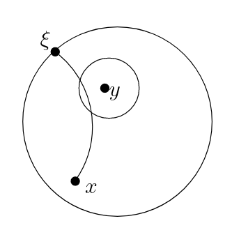
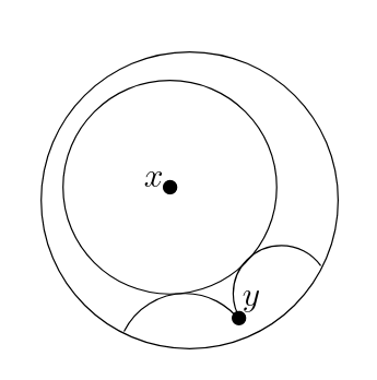
Definition (Shadow): For any points \(x\) in \(\overline{\mathbb{H}^2}\) and \(y\) in \(\mathbb{H}^2\), and any \(r \geq 0\), the shadow \(\mathcal{O}_r(x, y)\) is the set of all points \(\xi\) in \(\partial \mathbb{H}^2\) such that the geodesic from \(x\) to \(\xi\) intersects a ball of radius \(r\) around \(y\).
 |
Lemma (Sullivan's shadow lemma): Let \(\Gamma\) be a non-elementary discrete group, and let \(\{\mu_x\}_{x \in \mathbb{H}^2}\) be a \(\Gamma\)-invariant conformal density of dimension \(\delta\). Then for any \(x\) there exists a large enough \(r_0\), such that for all \(r \geq r_0\), there exists a \(C > 0\), depending on \(r\) for which the following inequality holds for all \(\gamma \in \Gamma\).
Proof: The first thing we need to show is that there exists an \(r\) large enough, and an \(\varepsilon\) small enough such that the following inequality holds for all \(y \in \overline{\Omega}\).
As \(r\) gets larger, the set \( \mathcal{O}_r(y, x)\) gets larger as well, and contains everything but the endpoint of the geodesic from \(x\) to \(y\). That means the only way this inequality can fail to hold is if all the mass of \(\mu_x\) was concentrated at that point. But since \(\Gamma\) is non-elementary, the measure \(\mu_x\) cannot be supported on a single point.
 |
We now rewrite \(\mu_x\left( \mathcal{O}_r(x, \gamma x) \right)\) using identities \eqref{eq:1} and \eqref{eq:2}.
Since we already know \( \mu_x\left( \mathcal{O}_r(\gamma^{-1}x, x) \right)\) is between \(1\) and \(\varepsilon\), all we need to do is estimate the Busemann function on the shadow. We can do that using the triangle inequality, which gives us the following inequality.
Combining \eqref{eq:5}, \eqref{eq:6}, and \eqref{eq:7}, we get the inequality we need. \(\square\)
All this may seem like it has noting to do with counting, but in fact, we already have developed enough tools to get a rough asymptotic count of the orbit points for convex cocompact groups, but that will have to wait for the next post because I think this post is long enough already.
-
The limit set of a Fuchsian group, S.J. Patterson ↩↩
-
The density at infinity of a discrete group of hyperbolic motions, Dennis Sullivan ↩
-
The proof goes via the proof of the fact that the Bowen-Margulis measure is an ergodic measure for the geodesic flow. At this point, it's natural to ask why is the easiest proof of ergodicity of the \(\Gamma\)-action via the ergodicity of the geodesic flow. A somewhat unsatisfactory answer to that is that the geodesic flow and the Bowen-Margulis measure have structures that are compatible with each other: the geodesic flow has stable and unstable manifolds, and the Bowen-Margulis measure happens to decompose nicely along these foliations. ↩